Plots.jl/docs/qwt_examples.md

Examples for backend: qwt

• Supported arguments: args, axis, background_color, color, fillto, foreground_color, group, heatmap_c, kwargs, label, legend, linestyle, linetype, marker, markercolor, markersize, nbins, reg, ribbon, show, size, title, width, windowtitle, xlabel, xticks, ylabel, yrightlabel, yticks
• Supported values for axis: :auto, :left, :right
• Supported values for linetype: :none, :line, :path, :steppre, :steppost, :sticks, :scatter, :heatmap, :hexbin, :hist, :bar
• Supported values for linestyle: :auto, :solid, :dash, :dot, :dashdot, :dashdotdot
• Supported values for marker: :none, :auto, :rect, :ellipse, :diamond, :utriangle, :dtriangle, :cross, :xcross, :star1, :star2, :hexagon
• Is subplot/subplot! supported? Yes

Initialize

using Plots
qwt!()

Lines

A simple line plot of the 3 columns.

plot(rand(50,5),w=3)

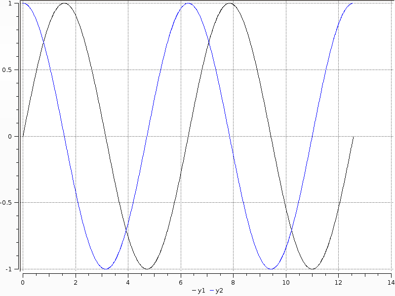
Functions

Plot multiple functions. You can also put the function first.

plot(0:0.01:4π,[sin,cos])

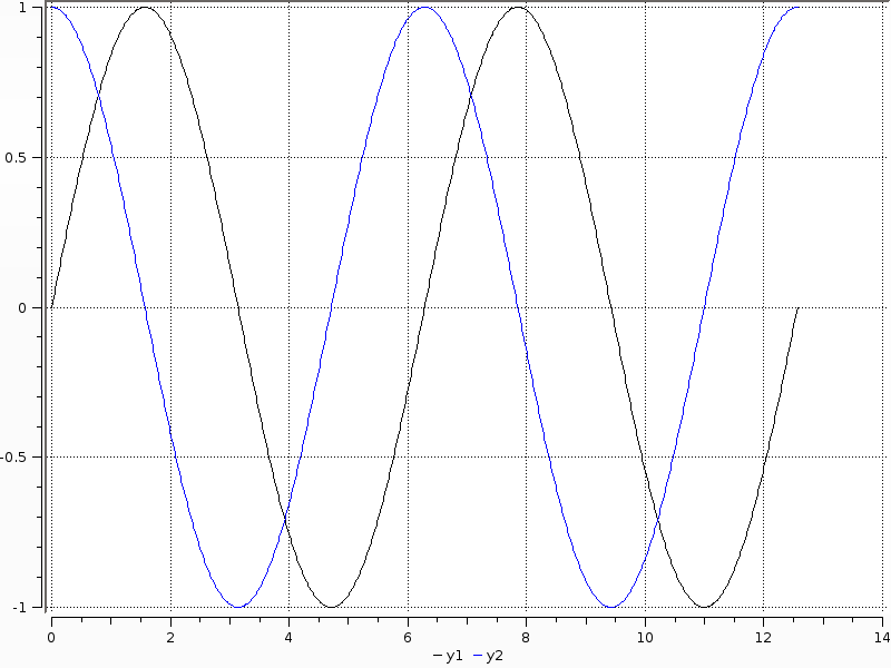
You can also call it with plot(f, xmin, xmax).

plot([sin,cos],0,4π)

Or make a parametric plot (i.e. plot: (fx(u), fy(u))) with plot(fx, fy, umin, umax).

plot(sin,(x->begin  # /home/tom/.julia/v0.4/Plots/docs/example_generation.jl, line 33:
            sin(2x)
        end),0,2π,legend=false,fillto=0)

Global

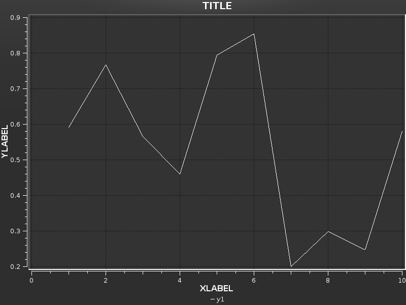
Change the guides/background without a separate call.

plot(rand(10); title="TITLE",xlabel="XLABEL",ylabel="YLABEL",background_color=RGB(0.2,0.2,0.2))

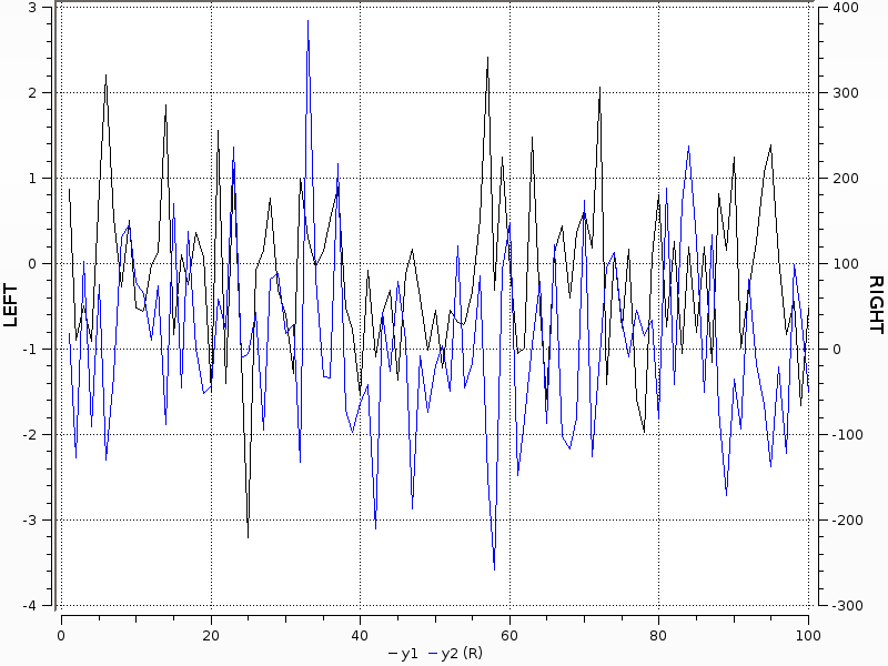
Two-axis

Use the axis or axiss arguments.

Note: Currently only supported with Qwt and PyPlot

plot(Vector[randn(100),randn(100) * 100]; axis=[:l,:r],ylabel="LEFT",yrightlabel="RIGHT")

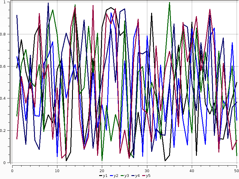
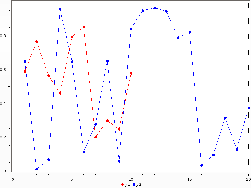
Vectors w/ pluralized args

Plot multiple series with different numbers of points. Mix arguments that apply to all series (singular... see marker) with arguments unique to each series (pluralized... see colors).

plot(Vector[rand(10),rand(20)]; marker=:ellipse,markersize=8,colors=[:red,:blue])

Build plot in pieces

Start with a base plot...

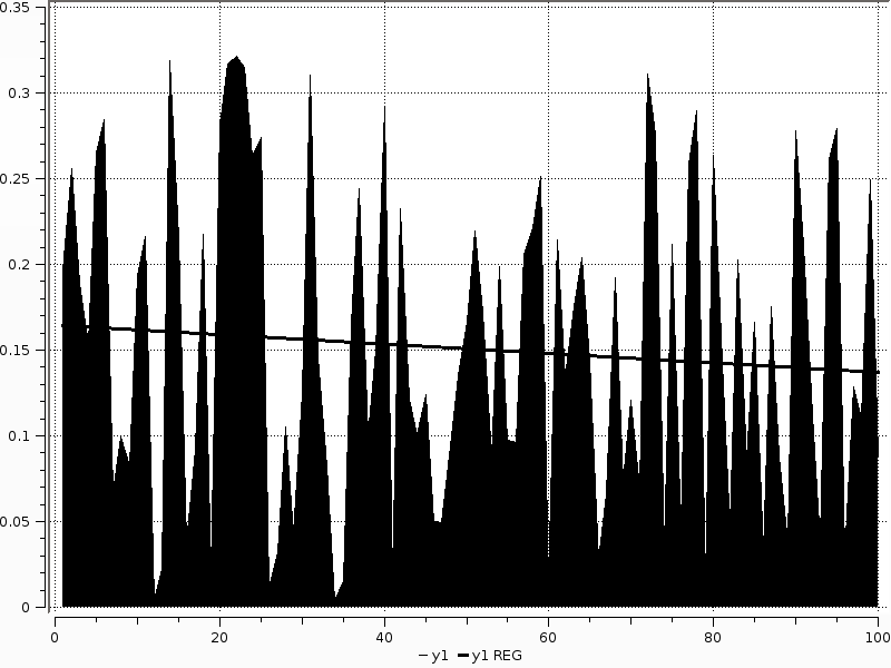
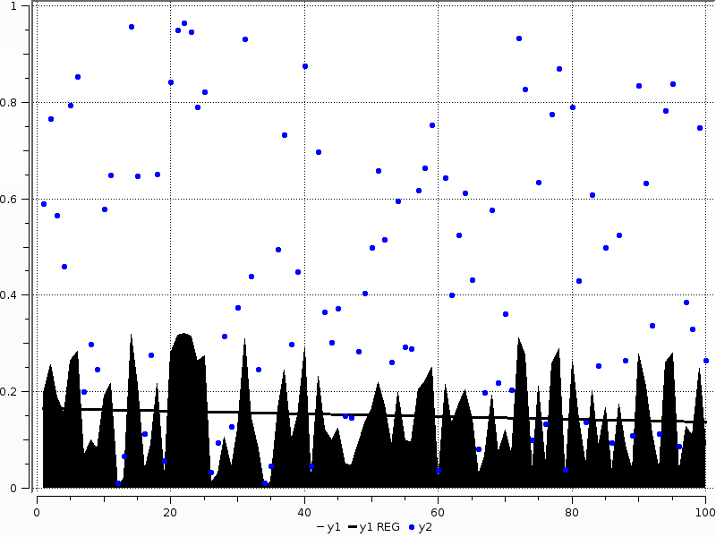
plot(rand(100) / 3; reg=true,fillto=0)

and add to it later.

scatter!(rand(100); markersize=6,c=:blue)

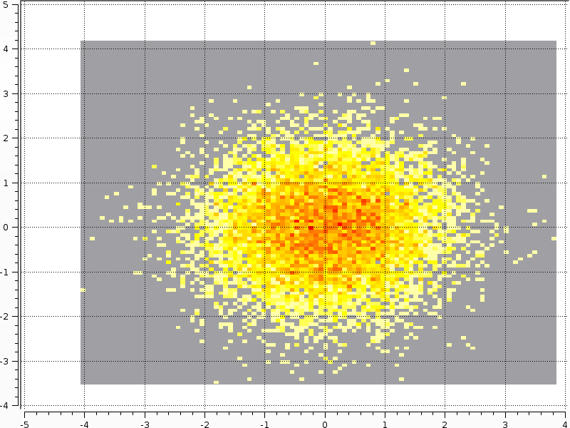
Heatmaps

heatmap(randn(10000),randn(10000); nbins=100)

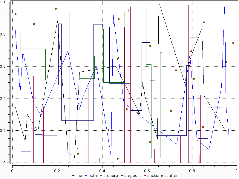
Line types

types = intersect(supportedTypes(),[:line,:path,:steppre,:steppost,:sticks,:scatter])
n = length(types)
x = Vector[sort(rand(20)) for i = 1:n]
y = rand(20,n)
plot(x,y; t=types,lab=map(string,types))

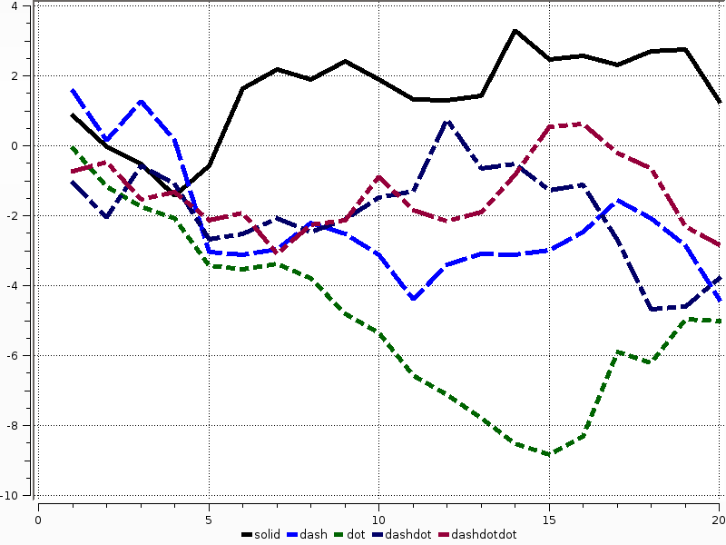
Line styles

styles = setdiff(supportedStyles(),[:auto])
plot(cumsum(randn(20,length(styles)),1); style=:auto,label=map(string,styles),w=5)

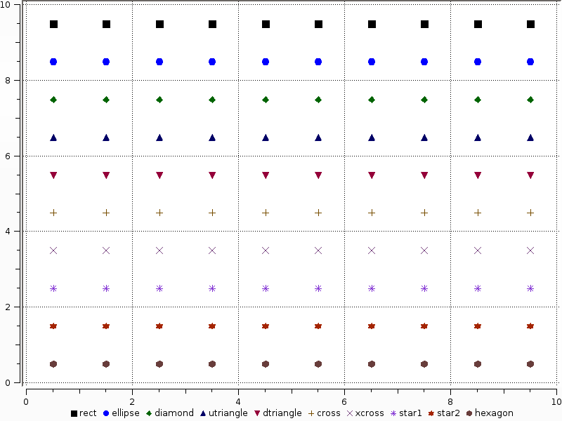
Marker types

markers = setdiff(supportedMarkers(),[:none,:auto])
scatter(0.5:9.5,[fill(i - 0.5,10) for i = length(markers):-1:1]; marker=:auto,label=map(string,markers),markersize=10)

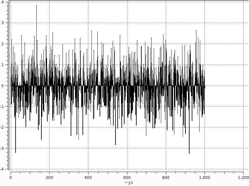
Bar

x is the midpoint of the bar. (todo: allow passing of edges instead of midpoints)

bar(randn(1000))

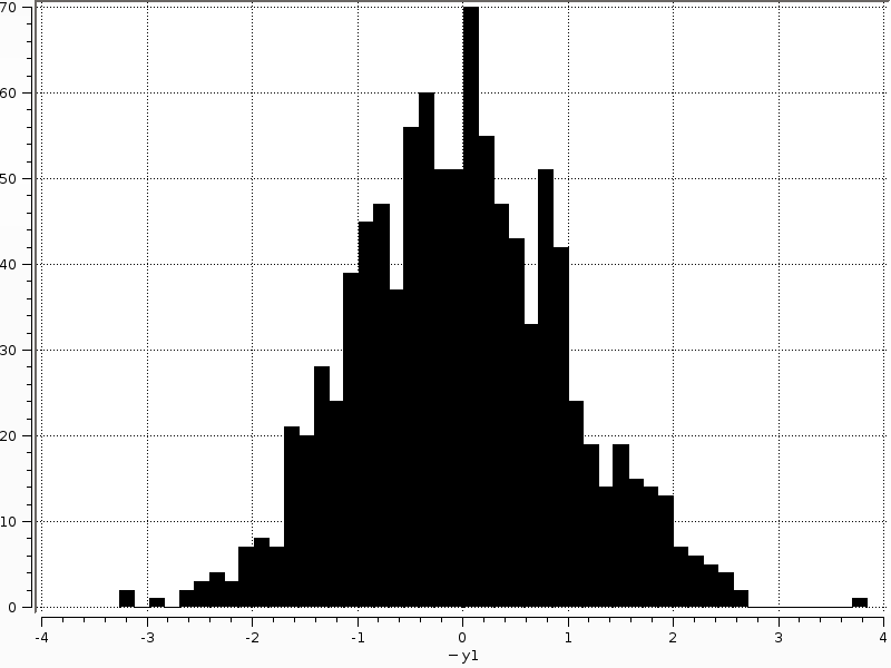
Histogram

histogram(randn(1000); nbins=50)

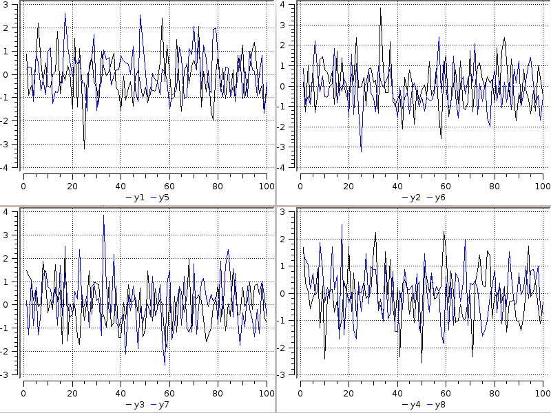
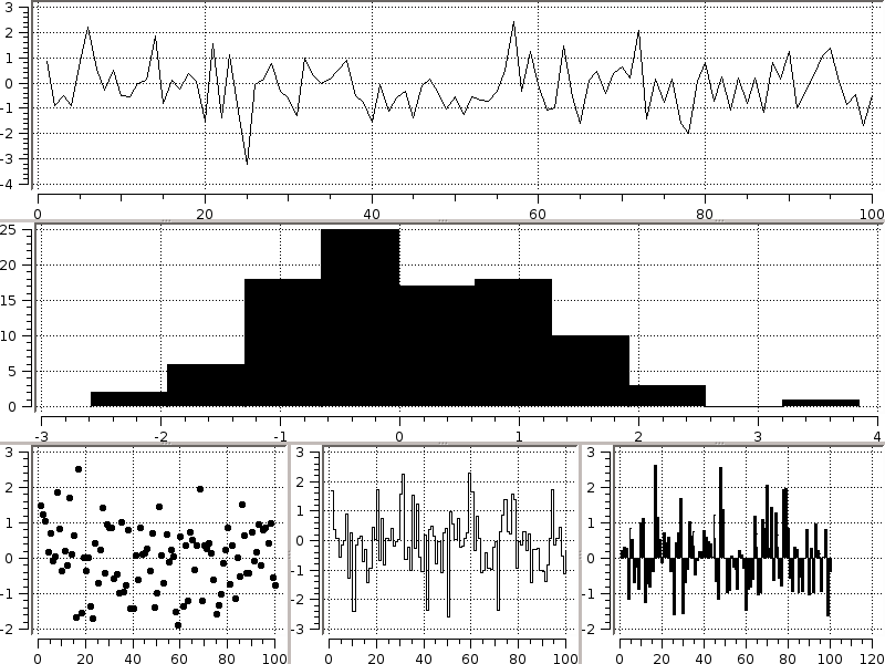
Subplots

subplot and subplot! are distinct commands which create many plots and add series to them in a circular fashion. You can define the layout with keyword params... either set the number of plots n (and optionally number of rows nr or number of columns nc), or you can set the layout directly with layout.

Note: Gadfly is not very friendly here, and although you can create a plot and save a PNG, I haven't been able to actually display it.

subplot(randn(100,5); layout=[1,1,3],linetypes=[:line,:hist,:scatter,:step,:bar],nbins=10,legend=false)

Adding to subplots

Note here the automatic grid layout, as well as the order in which new series are added to the plots.

subplot(randn(100,5); n=4)

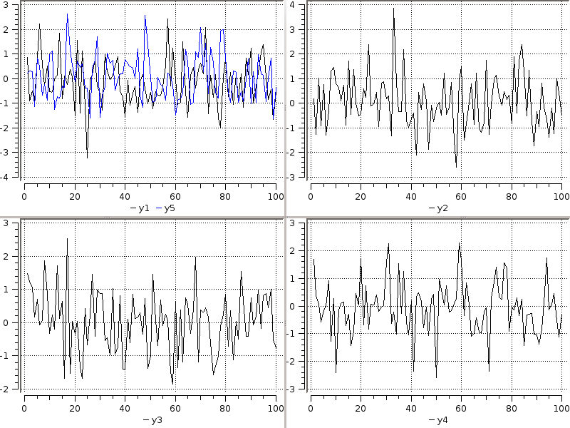
subplot!(randn(100,3))