Gnuplot.jl

A Julia interface to gnuplot.

Gnuplot.jl is a simple package able to send both data and commands from Julia to an underlying gnuplot process. Its main purpose it to provide a fast and powerful data visualization framework, using an extremely concise Julia syntax. It also has automatic display of plots in Jupyter, Juno and VS Code.

Installation

Install with:

]add Gnuplot

A working gnuplot package must be installed on your platform.

You may check the installed Gnuplot.jl version with:

]st Gnuplot

If the displayed version is not v1.4.0 you are probably having a dependency conflict. In this case try forcing installation of the latest version with:

]add Gnuplot@1.4.0

and check which package is causing the conflict.

Test package:

using Gnuplot
println(Gnuplot.gpversion())
test_terminal()

Quick start

The following examples are supposed to be self-explaining. See documentation for further informations.

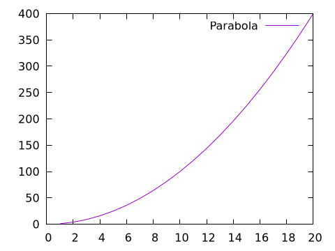
A simple parabola

x = 1.:20
@gp x x.^2 "with lines title 'Parabola'"
save(term="pngcairo size 480,360", output="examples/ex1.png")
save("parabola.gp")  # => save a script file with both data and command to re-create the plot.

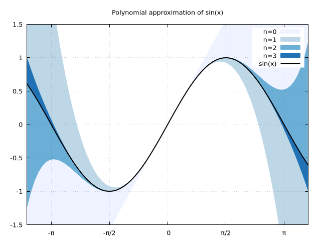
A slightly more complex plot, with unicode on X tics

x = -2pi:0.1:2pi
approx = fill(0., length(x));
@gp tit="Polynomial approximation of sin(x)" key="opaque" linetypes(:Blues_4)
@gp :- "set encoding utf8" raw"""set xtics ('-π' -pi, '-π/2' -pi/2, 0, 'π/2' pi/2, 'π' pi)"""
@gp :- xr=3.8.*[-1, 1] yr=[-1.5,1.5] "set grid front"
@gp :- x sin.(x) approx .+=  x          "w filledcurve t 'n=0' lt 1"
@gp :- x sin.(x) approx .+= -x.^3/6     "w filledcurve t 'n=1' lt 2"
@gp :- x sin.(x) approx .+=  x.^5/120   "w filledcurve t 'n=2' lt 3"
@gp :- x sin.(x) approx .+= -x.^7/5040  "w filledcurve t 'n=3' lt 4"
@gp :- x sin.(x)                        "w l t 'sin(x)' lw 2 lc rgb 'black'"
save(term="pngcairo size 640,480", output="examples/ex2.png")

Multiplot: a 2D histogram contour plot and a 3D surface plot

x = randn(10_000)
y = randn(10_000)
h = hist(x, y, bs1=0.25, nbins2=20)
@gp "set multiplot layout 1,2"
@gp :- 1 key="outside top center box horizontal" "set size ratio -1" h
clines = contourlines(h, "levels discrete 10, 30, 60, 90");
for i in 1:length(clines)
    @gp :- clines[i].data "w l t '$(clines[i].z)' lw $i lc rgb 'gray'" :-
end
@gsp :- 2 h.bins1 h.bins2 h.counts "w pm3d notit"
save(term="pngcairo size 660,350 fontscale 0.8", output="examples/ex3.png")

Further examples

The main gallery of examples is maintained in a separate repository: https://lazarusa.github.io/gnuplot-examples/

Since Gnuplot.jl is just a transparent interface (not a wrapper) it exposes all capabilities of the underlying gnuplot process, hence pure-gnuplot examples also applies to Gnuplot.jl. Further examples are available here:

• http://gnuplot.sourceforge.net/demo_5.2/
• http://www.gnuplotting.org/