When the plot pane is disabled, VS Code neither shows the plot nor
prints any warning/error. The plot is not shown because Gnuplot.jl
thinks the VS Code can display it. We fix that by adding a check for
whether the pane is enabled.

This is not an ideal solution because the check is executed only when
loading Gnuplot.jl. If the panel is disabled later in the REPL
session, no plots will be shown. If this turns out to be a problem, we
will need to extend `showable` and perform the check there.

The problem of not showing a warning/error when the plot pane is
disabled must be addressed in julia-vscode. It seems that the Plots
package doesn't produce any warning/error in this case too.

Related to #45.
Gnuplot.jl
A Julia interface to gnuplot.

![]()
![]()
Gnuplot.jl is a simple package able to send both data and commands from Julia to an underlying gnuplot process. Its main purpose it to provide a fast and powerful data visualization framework, using an extremely concise Julia syntax. It also has automatic display of plots in Jupyter, Juno and VS Code.
Installation
Install with:
]add Gnuplot
A working gnuplot package must be installed on your platform.
You may check the installed Gnuplot.jl version with:
]st Gnuplot
If the displayed version is not v1.4.0 you are probably having a dependency conflict. In this case try forcing installation of the latest version with:
]add Gnuplot@1.4.0
and check which package is causing the conflict.
Test package:
using Gnuplot
println(Gnuplot.gpversion())
test_terminal()
Quick start
The following examples are supposed to be self-explaining. See documentation for further informations.
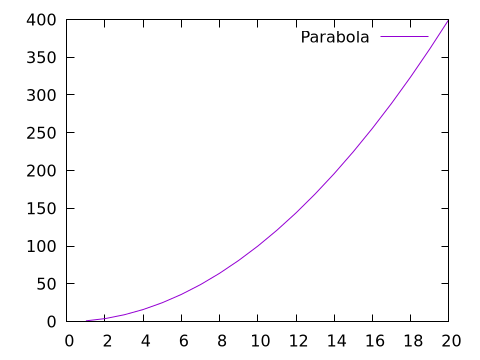
A simple parabola
x = 1.:20
@gp x x.^2 "with lines title 'Parabola'"
save(term="pngcairo size 480,360", output="examples/ex1.png")
save("parabola.gp")  # => save a script file with both data and command to re-create the plot.
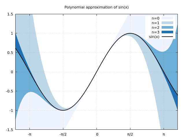
A slightly more complex plot, with unicode on X tics
x = -2pi:0.1:2pi
approx = fill(0., length(x));
@gp tit="Polynomial approximation of sin(x)" key="opaque" linetypes(:Blues_4)
@gp :- "set encoding utf8" raw"""set xtics ('-π' -pi, '-π/2' -pi/2, 0, 'π/2' pi/2, 'π' pi)"""
@gp :- xr=3.8.*[-1, 1] yr=[-1.5,1.5] "set grid front"
@gp :- x sin.(x) approx .+=  x          "w filledcurve t 'n=0' lt 1"
@gp :- x sin.(x) approx .+= -x.^3/6     "w filledcurve t 'n=1' lt 2"
@gp :- x sin.(x) approx .+=  x.^5/120   "w filledcurve t 'n=2' lt 3"
@gp :- x sin.(x) approx .+= -x.^7/5040  "w filledcurve t 'n=3' lt 4"
@gp :- x sin.(x)                        "w l t 'sin(x)' lw 2 lc rgb 'black'"
save(term="pngcairo size 640,480", output="examples/ex2.png")
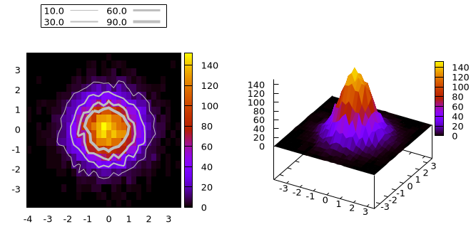
Multiplot: a 2D histogram contour plot and a 3D surface plot
x = randn(10_000)
y = randn(10_000)
h = hist(x, y, bs1=0.25, nbins2=20)
@gp "set multiplot layout 1,2"
@gp :- 1 key="outside top center box horizontal" "set size ratio -1" h
clines = contourlines(h, "levels discrete 10, 30, 60, 90");
for i in 1:length(clines)
    @gp :- clines[i].data "w l t '$(clines[i].z)' lw $i lc rgb 'gray'" :-
end
@gsp :- 2 h.bins1 h.bins2 h.counts "w pm3d notit"
save(term="pngcairo size 660,350 fontscale 0.8", output="examples/ex3.png")
Further examples
The main gallery of examples is maintained in a separate repository: https://lazarusa.github.io/gnuplot-examples/
Since Gnuplot.jl is just a transparent interface (not a wrapper) it exposes all capabilities of the underlying gnuplot process, hence pure-gnuplot examples also applies to Gnuplot.jl. Further examples are available here: