Advanced usage

Here we will show a few advanced techniques for data visualization using Gnuplot.jl.

Named datasets

A dataset may have an associated name whose purpose is to use it multiple times for plotting, while sending it only once to gnuplot. A dataset name must begin with a $.

A named dataset is defined as a Pair{String, Tuple}, e.g.:

"\$name" => (1:10,)

and can be used as an argument to both @gp and gsp, e.g.:

x = range(-2pi, stop=2pi, length=100);
y = sin.(x)
name = "\$MyDataSet1"
@gp name=>(x, y) "plot $name w l lc rgb 'black'" "pl $name u 1:(1.5*\$2) w l lc rgb 'red'"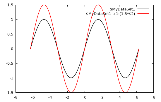

Both curves use the same input data, but the red curve has the second column (\$2, corresponding to the y value) multiplied by a factor 1.5.

A named dataset comes in hand also when using gnuplot to fit experimental data to a model, e.g.:

# Generate data and some noise to simulate measurements
x = range(-2pi, stop=2pi, length=20);
y = 1.5 * sin.(0.3 .+ 0.7x);
err = 0.1 * maximum(abs.(y)) .* fill(1, size(x));
y += err .* randn(length(x));
name = "\$MyDataSet1"

@gp    "f(x) = a * sin(b + c*x)"     :- # define an analytical model
@gp :- "a=1" "b=1" "c=1"             :- # set parameter initial values
@gp :- name=>(x, y, err)             :- # define a named dataset
@gp :- "fit f(x) $name via a, b, c;"    # fit the data

The parameter best fit values can be retrieved as follows:

vars = gpvars();
@info("Best fit values:",
  a = vars.a,
  b = vars.b,
  c = vars.c)

┌ Info: Best fit values:
│   a = 1.53507096513964
│   b = 0.333804739506457
└   c = 0.701159811567446

Multiplot

Gnuplot.jl can draw multiple plots in the same figure by exploiting the multiplot command. Each plot is identified by a positive integer number, which can be used as argument to @gp to redirect commands to the appropriate plot.

Recycling data from the previous example we can plot both data and best fit model (in plot 1) and residuals (in plot 2):

@gp    "f(x) = a * sin(b + c*x)"
@gp :- "a=$(vars.a)" "b=$(vars.b)" "c=$(vars.c)"
@gp :- name=>(x, y, err)
@gp :- "set multiplot layout 2,1"
@gp :- 1 "p $name w errorbars t 'Data'"
@gp :-   "p $name u 1:(f(\$1)) w l t 'Best fit model'"
@gp :- 2 "p $name u 1:((f(\$1)-\$2) / \$3):(1) w errorbars t 'Resid. [{/Symbol s}]'"
@gp :-   [extrema(x)...] [0,0] "w l notit dt 2 lc rgb 'black'" # reference line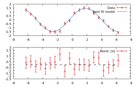

Note that the order of the plots is not relevant, i.e. we would get the same results with:

@gp    "f(x) = a * sin(b + c*x)"
@gp :- "a=$(vars.a)" "b=$(vars.b)" "c=$(vars.c)"
@gp :- name=>(x, y, err)
@gp :- "set multiplot layout 2,1"
@gp :- 2 "p $name u 1:((f(\$1)-\$2) / \$3):(1) w errorbars t 'Resid. [{/Symbol s}]'"
@gp :-   [extrema(x)...] [0,0] "w l notit dt 2 lc rgb 'black'" # reference line
@gp :- 1 "p $name w errorbars t 'Data'"
@gp :-   "p $name u 1:(f(\$1)) w l t 'Best fit model'"

Customized layout

It is also possible to customize the plot layout using the margin keywords (see Histograms for further info):

# Generate random numbers
x = randn(1000);
y = randn(1000);

# Overall plot margins (normalized in the range 0:1)
margins = (l=0.08, r=0.98, b=0.13, t=0.98)

# Right and top margins of main plot
right, top = 0.8, 0.75

# Gap between main plot and histograms
gap  = 0.015

# Main plot
@gp "set multiplot"
@gp :- 1 ma=margins rma=right tma=top :-
@gp :-   x y "w p notit" xlab="X" ylab="Y"
xr = gpranges().x  # save current X range
yr = gpranges().y  # save current Y range

# Histogram on X
h = hist(x, nbins=10)
@gp :- 2 ma=margins bma=top+gap rma=right :-
@gp :-   "set xtics format ''" "set ytics format ''"  xlab="" ylab="" :-
bs = fill(h.binsize, length(h.bins));
@gp :-   xr=xr h.bins h.counts./2 bs./2 h.counts./2 "w boxxy notit fs solid 0.4" :-

# Histogram on Y
h = hist(y, nbins=10)
@gp :- 3 ma=margins lma=right+gap tma=top :-
@gp :-     "unset xrange" :-
bs = fill(h.binsize, length(h.bins));
@gp :-   yr=yr h.counts./2 h.bins h.counts./2 bs./2 "w boxxy notit fs solid 0.4" :-
@gp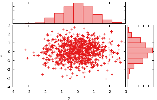

Mixing 2D and 3D plots

A multiplot can also mix 2D and 3D plots:

x = y = -10:0.33:10
@gp "set multiplot layout 1,2"

# 2D
@gp :- 1 x sin.(x) ./ x "w l notit"

# 3D
sinc2d(x,y) = sin.(sqrt.(x.^2 + y.^2))./sqrt.(x.^2+y.^2)
fxy = [sinc2d(x,y) for x in x, y in y]
@gsp :- 2 x y fxy "w pm3d notit"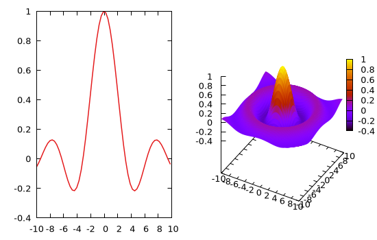

Multiple sessions

Gnuplot.jl can handle multiple sessions, i.e. multiple gnuplot processes running simultaneously. Each session is identified by an ID (sid::Symbol, in the documentation).

In order to redirect commands to a specific session simply insert a symbol into your @gp or @gsp call, e.g.:

@gp :GP1 "plot sin(x)"    # opens first window
@gp :GP2 "plot sin(x)"    # opens secondo window
@gp :- :GP1 "plot cos(x)" # add a plot on first window

The session ID can appear in every position in the argument list, but only one ID can be present in each call. If the session ID is not specified the :default session is used.

The names of all current sessions can be retrieved with session_names():

julia> println(session_names())
[:default, :GP1, :GP2]

To quit a specific session use Gnuplot.quit():

julia> Gnuplot.quit(:GP1)
0

The output value is the exit status of the underlying gnuplot process.

You may also quit all active sessions at once with Gnuplot.quitall():

julia> Gnuplot.quitall()

Histograms

Gnuplot.jl provides a facility to compute (see hist() function) an histogram. It allows to set the range to consider (range= keyword) and either the bin size (bs=) or the total number of bins (nbins=) in the histogram (see hist() documentation for further information) and return a Gnuplot.Histogram1D structure, whose content can be visualized as follows:

x = randn(1000);
h = hist(x, range=3 .* [-1,1], bs=0.5)
@gp h.bins h.counts "w histep t 'Data' lc rgb 'red'"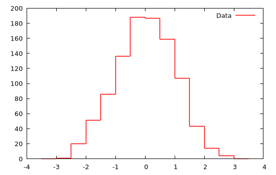

Gnuplot.jl also allows to compute 2D histograms by passing two vectors (with the same lengths) to hist(). Again, a finer control can be achieved by specifying ranges, bin size or number of bins (along both dimensions) and by explicitly using the content of the returned Gnuplot.Histogram2D structure:

x = randn(10_000)
y = randn(10_000)
h = hist(x, y, bs1=0.25, nbins2=20, range1=[-3,3], range2=[-3,3])
@gp "set size ratio -1" h.bins1 h.bins2 h.counts "w image notit"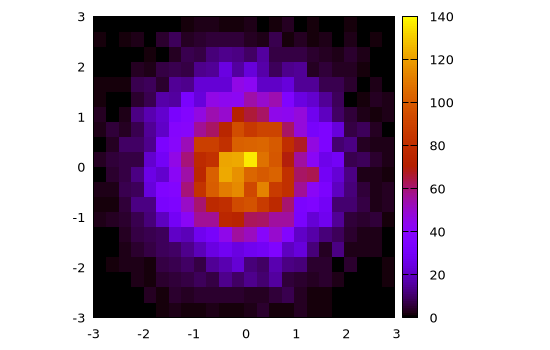

Alternatively, 2D histograms may be displayed using the boxxyerror plot style which allows more flexibility in, e.g., handling transparencies and drawing the histogram grid. In this case the data can be prepared using the boxxyerror() function, as follows:

box = boxxyerror(h.bins1, h.bins2, cartesian=true)
@gp "set size ratio -1" "set style fill solid 0.5 border lc rgb 'gray'" :-
@gp :- box... h.counts "w boxxyerror notit lc pal"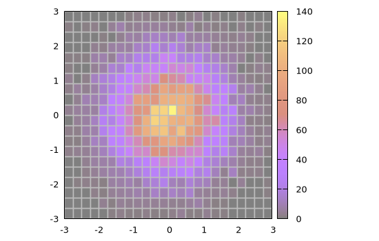

See also Histogram recipes for a quicker way to preview histogram plots.

Contour lines

Although gnuplot already handles contours by itself (with the set contour command), Gnuplot.jl provides a way to calculate contour lines paths before displaying them, using the contourlines() function. We may use it for, e.g., plot contour lines with customized widths and palette, according to their z level. Continuing with the previous example:

clines = contourlines(h.bins1, h.bins2, h.counts, cntrparam="levels discrete 10, 30, 60, 90");
for i in 1:length(clines)
    @gp :- clines[i].data "w l t '$(clines[i].z)' lw $i lc pal" :-
end
@gp :- key="outside top center box horizontal"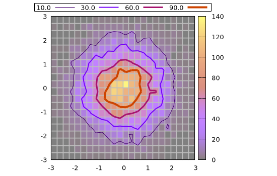

Animations

The Multiplot capabilities can also be used to stack plots one above the other in order to create an animation, as in the following example:

x = y = -10:0.33:10
fz(x,y) = sin.(sqrt.(x.^2 + y.^2))./sqrt.(x.^2+y.^2)
fxy = [fz(x,y) for x in x, y in y]
@gsp "set xyplane at 0" "unset colorbox" cbr=[-1,1] zr=[-1,1]
frame = 0
for direction in [-1,1]
    for factor in -1:0.1:1
        global frame += 1
        @gsp :- frame x y direction * factor .* fxy "w pm3d notit" :-
    end
end
@gsp

Here the frame variable is used as multiplot index. The animation can be saved in a GIF file with:

save(term="gif animate size 480,360 delay 5", output="assets/animation.gif")

Direct command execution

When gnuplot commands are passed to @gp or @gsp they are stored in a session for future use, or to be saved in Gnuplot scripts. If you simply wish to execute a command without storing it in the session, and possibly retrieve a value, use gpexec. E.g., to retrieve the value of a gnuplot variable:

julia> gpexec("print GPVAL_TERM")
"unknown"

You may also provide a session ID as first argument (see Multiple sessions) to redirect the command to a specific session.

Alternatively you may start the The gnuplot REPL to type commands directly from the Julia prompt.

The gnuplot REPL

The Gnuplot.jl package comes with a built-in REPL mode to directly send commands to the underlying gnuplot process. Since the REPL is a global resource, the gnuplot mode is not enabled by default. You can start it with:

Gnuplot.repl_init(start_key='>')

The customizable start_key character is the key which triggers activation of the REPL mode. To quit the gnuplot REPL mode hit the backspace key.

Dry sessions

A "dry session" is a session with no underlying gnuplot process. To enable dry sessions type:

Gnuplot.options.dry = true;

before starting a session (see also Options). Note that the dry option is a global one, i.e. it affects all sessions started after setting the option.

Clearly, no plot can be generated in dry sessions. Still, they are useful to run Gnuplot.jl code without raising errors (no attempt will be made to communicate with the underlying process). Moreover, Gnuplot scripts can also be generated in a dry session, without the additional overhead of sending data to the gnuplot process.

If a gnuplot process can not be started the package will print a warning, and automatically enable dry sessions.