Advanced techniques
Here we will show a few advanced techniques for data visualization using Gnuplot.jl. The new concepts introduced in the examples are as follows:
a name can be associated to a dataset, in order to use it multiple times in a plot while sending it only once to gnuplot. A dataset name must begin with a
$;gnuplot is able to generate multiplot, i.e. a single figure containing multiple plots. Each plot is identified by a numeric ID, starting from 1;
Gnuplot.jl is able to handle multiple sessions, i.e. multiple gnuplot processes running simultaneously. Each session is identified by a symbol. If the session ID is not specified the
:defaultsession is considered.
Named datasets
A named dataset can be used multiple times in a plot, avoiding sending to gnuplot the same data multiple times. A dataset name must always start with a $, and the dataset is defined as a Pair{String, Tuple}, e.g.:
"\$name" => (1:10,)A named dataset can be used as an argument to both @gp and gsp, e.g.:
x = range(-2pi, stop=2pi, length=100);
y = sin.(x)
name = "\$MyDataSet1"
@gp name=>(x, y) "plot $name w l lc rgb 'black'" "pl $name u 1:(-1.5*\$2) w l lc rgb 'red'"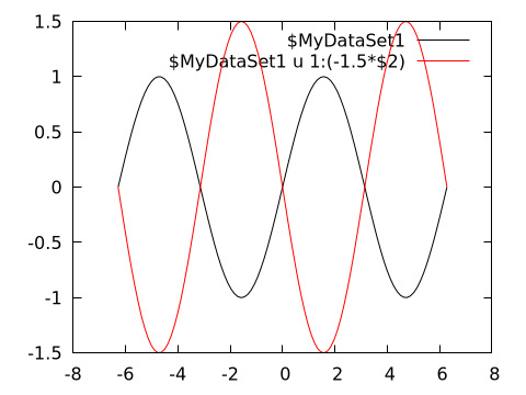
Both curves use the same input data, but the red curve has the second column (\$2, corresponding to the y value) is multiplied by a factor -1.5.
A named dataset comes in hand also when using gnuplot to fit experimental data to a model, e.g.:
# Generate data and some noise to simulate measurements
x = range(-2pi, stop=2pi, length=20);
y = 1.5 * sin.(0.3 .+ 0.7x);
err = 0.1 * maximum(abs.(y)) .* fill(1, size(x));
y += err .* randn(length(x));
name = "\$MyDataSet1"

@gp    "f(x) = a * sin(b + c*x)"     :- # define an analytical model
@gp :- "a=1" "b=1" "c=1"             :- # set parameter initial values
@gp :- name=>(x, y, err)             :- # define a named dataset
@gp :- "fit f(x) $name via a, b, c;"    # fit the data
The parameter best fit values can be retrieved as follows:
@info("Best fit values:",
a=Gnuplot.exec("print a"),
b=Gnuplot.exec("print b"),
c=Gnuplot.exec("print c"))
┌ Info: Best fit values:
│ a = "1.49753503068311"
│ b = "0.265280323129744"
└ c = "0.695848802236574"A named dataset is available until the session is reset, i.e. as long as :- is used as first argument to @gp.
Multiplot
Gnuplot.jl can draw multiple plots in the same figure by exploiting the multiplot command. Each plot is identified by a positive integer number, which can be used as argument to @gp to redirect commands to the appropriate plot.
Continuing previous example we can plot both data and best fit model (in plot 1) and residuals (in plot 2):
@gp :- "set multiplot layout 2,1"
@gp :- 1 "p $name w errorbars t 'Data'"
@gp :-   "p $name u 1:(f(\$1)) w l t 'Best fit model'"
@gp :- 2 "p $name u 1:((f(\$1)-\$2) / \$3):(1) w errorbars t 'Resid. [{/Symbol s}]'"
@gp :-   [extrema(x)...] [0,0] "w l notit dt 2 lc rgb 'black'" # reference line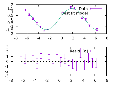
Note that the order of the plots is not relevant, i.e. we would get the same results with:
@gp :- "set multiplot layout 2,1"
@gp :- 2 "p $name u 1:((f(\$1)-\$2) / \$3):(1) w errorbars t 'Resid. [{/Symbol s}]'"
@gp :-   [extrema(x)...] [0,0] "w l notit dt 2 lc rgb 'black'" # reference line
@gp :- 1 "p $name w errorbars t 'Data'"
@gp :-   "p $name u 1:(f(\$1)) w l t 'Best fit model'"
Mixing 2D and 3D plots
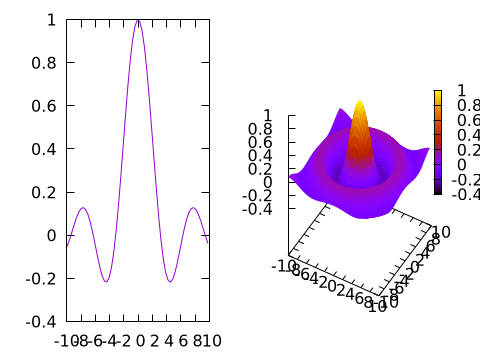
A multiplot can also mix 2D and 3D plots:
x = y = -10:0.33:10
@gp "set multiplot layout 1,2"

# 2D
@gp :- 1 x sin.(x) ./ x "w l notit"

# 3D
sinc2d(x,y) = sin.(sqrt.(x.^2 + y.^2))./sqrt.(x.^2+y.^2)
fxy = [sinc2d(x,y) for x in x, y in y]
@gsp :- 2 x y fxy "w pm3d notit"